Measuring and Monitoring Arrow's Performance: Some Updated R Benchmarks

The Apache Arrow project defines a standardized, language-agnostic, columnar data format optimized for speed and efficiency. But a fast in-memory format is valuable only if you can read data into it and write data out of it, so Arrow libraries include methods for working with common file formats including CSV, JSON, and Parquet, as well as Feather, which is Arrow on disk. By using Arrow libraries, developers of analytic data systems can avoid the hassle of implementing their own methods for reading and writing data in these formats.

Because the Arrow format is designed for fast and efficient computation, users of Arrow libraries have high expectations for performance. Of course, it’s unrealistic to expect any one piece of software to be fastest at everything—software design involves tradeoffs and optimizing for certain use cases over others. That said, we should expect that Arrow libraries can take advantage of modern hardware features like SIMD and be efficient with memory, and this should result in good performance.

We’ve done some ad hoc benchmarking in the past that has shown how Arrow libraries measure up on certain workloads. This has demonstrated, among other things, the speed and efficiency of reading and writing Parquet and Feather files, how Arrow’s CSV reader compares with alternatives in R, and how fast we can execute a query over 1.5 billion rows of data partitioned into lots of Parquet files.

These results are interesting—sometimes provocative—but they have limitations. For one, they’re snapshots: they give us a result that corresponds to a particular version of the code, but they don’t tell us how performance evolves over time—whether our changes have made things faster or slower. They also are time- and labor-intensive to set up, so we haven’t done them as often as we should, and we’ve been limited in the kinds of questions we could answer.

We’ve recently been investing in tools and infrastructure to solve these problems. Our goal is to elevate performance monitoring to a similar position as unit testing is in our continuous integration stack. Since speed is a key feature of Arrow, we should test it regularly and use benchmarking to prevent performance regressions. And just as one invests in tooling to make it easy to write and run tests—so that developers will be encouraged to write more tests—we’re working to improve the experience of writing and running benchmarks.

We’ll talk more about the continuous benchmarking and monitoring project in a future post. Here, we wanted to revisit some R benchmark results we’ve presented in the past, see how they hold up with the latest versions of the code, and discuss some of the research and insights we’ve been able to pursue thanks to our new tools.

The {arrowbench} package

To help us investigate and monitor performance in R, we’ve been developing a package called {arrowbench}¹. It contains tools for defining benchmarks, running them across a range of parameters, and reporting their results in a standardized form. The goal is to make it easier for us to test different library versions, variables, and machines, as well as to facilitate continuous monitoring.

While this package could be used for microbenchmarking, it is designed specially for “macrobenchmarks”: workflows that real users do with real data that take longer than milliseconds to run. It builds on top of existing R benchmarking tools, notably the {bench} package. Among the features that this package adds are

• Setup designed with parametrization in mind so you can test across a range of variables
• Isolation of benchmark runs in separate processes to prevent cross-contamination such as global environment changes and previous memory allocation
• Tools for bootstrapping package versions and known data sources to facilitate running the same code on different machines

While we’ve put work into {arrowbench} for a while now, it is a work in progress and we anticipate it will grow, change, and improve over time. Even so, in its current state, it’s enabled us to ask and answer performance-related questions we could not previously explore.

Revisiting CSV reading benchmarks

At the New York R Conference in August 2020, Neal presented results from extending the benchmark suite in the {vroom} package to include variations using {arrow} and {cudf}, a Python package based on Apache Arrow that runs on GPUs. {vroom}’s benchmarks are great for a number of reasons: they run on a range of datasets with different sizes, shapes, and data types, including using real-world data and not just synthetic, generated files; they’re honest—{vroom} isn’t fastest everywhere; and they’re scripted and well documented, easily reproducible and extensible.

While it was not the primary result of focus for the presentation, this plot showing the time it took to read a CSV into a fully materialized R data.frame got a lot of attention:

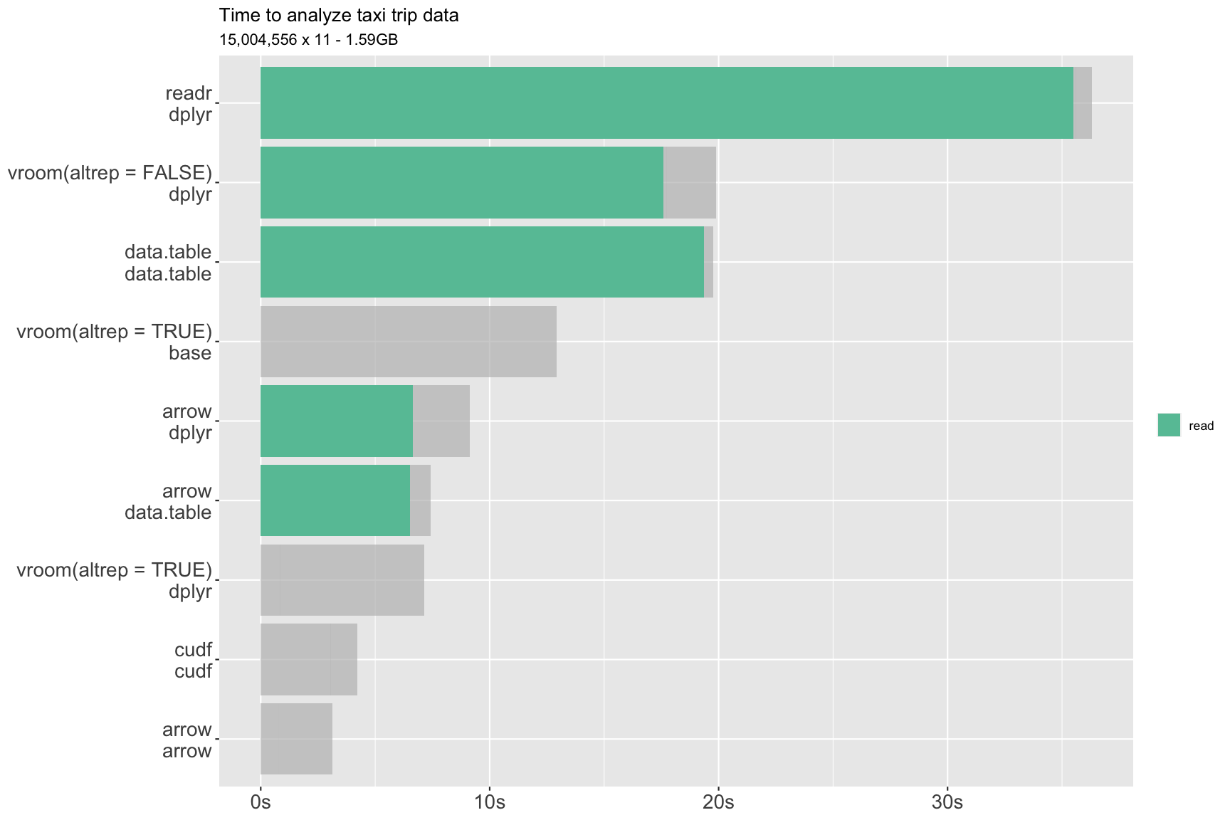
The green bars indicate the time to read the CSV into a data.frame using the reader on the first line of the legend ({readr}, etc.); gray bars extending beyond the green are the time spent on later stages of the benchmarked workflow (printing, sampling rows, computing a grouped aggregation) using the package on the second line of the legend (e.g. {dplyr}). Fully gray bars with no green are benchmark variations that don’t pull all of the data into a data.frame: {vroom} with altrep = TRUE, for example, doesn’t have to read all of the data in in order to complete the rest of the test workflow.

In sum, the plot showed that using {arrow} just for its CSV reader could provide 2-3x speedups compared to other readers, at least on files like this one with millions of rows and including string columns. Once you had used {arrow} to read the data into a data.frame, you could then use your preferred R analytics packages on the data—there was nothing special or Arrow-flavored about the data.frame it produced.

This seemed like an interesting result to revisit and track over time, so we added it to our new benchmarking framework. We now have a benchmark for CSV reading with several parameters:

• Files: we’re using the same two test datasets we used in our previous analysis of Feather and Parquet reading:

  • The 2016 Q4 Fannie Mae Loan Performance dataset, which is a 1.52 GB pipe-delimited file
    • 22 million rows by 31 columns
    • Column types are 18 numerics (of which 6 are integers), 11 characters, and 2 columns with no values at all
  • The January 2010 NYC Yellow Taxi Trip Records file, which is a 2.54 GB CSV
    • Nearly 15 million rows by 18 columns
    • Column types are 14 numerics (none of which are integers), 2 datetimes, and 2 characters

  We are using these datasets because they are the kind of datasets that people use in real life, including string columns, dates, fully empty columns, and missing data.

• Reader: we compare arrow::read_csv_arrow() with data.table::fread(), readr::read_csv(), and vroom::vroom(). vroom() is called with altrep = FALSE in this benchmark because we’re comparing how long it takes to read the data into memory as an R data.frame. With the exception of providing the delimiter to each, we are using the defaults for the arguments on all reading functions.

• Result: contrary to the previous statement, for the {arrow} reader only, we benchmark both how long it takes to read an Arrow Table as well as an R data.frame. Because {arrow}’s readers work by first reading the file into an Arrow Table and then converting the Table to a data.frame, comparing these two results tells us the relative speed of those two sections of work, and thus where we might focus our attention for performance optimization.²

• Compression: uncompressed or gzipped. The Fannie Mae file is 208 MB when gzipped; the taxi file, 592 MB. All four CSV reading functions can read both compressed and uncompressed files.

• CPU/thread count: we can flexibly test how these readers perform with different numbers of threads available for parallelization. Note that {readr} is only single-threaded, so we exclude it from the multithreaded results.

We can also test across a range of library versions, which we’ll show below.

Initial results

Using {arrowbench}, we have recreated benchmarks similar to those from the August 2020 presentation, isolating the CSV-read-to-data-frame portion. Code to run the benchmarks and generate the plots below, along with the data we collected (in both Parquet and CSV format), are available.

The results here are from a MacBook Pro with a 2GHz Quad-Core Intel Core i5 and 16 GB of RAM, though we also ran them on a MacPro with a 3.5 GHz 6-Core Intel Xeon E5 and 64GB of RAM and a system with a 4.5 GHz Quad-Core Intel Core i7 and 32GB of RAM running Ubuntu 18.04. We saw broadly similar results across each of these machines, but included only one system for clarity.³

We are looking at out-of-the-box performance, not some sort of theoretical ideal performance. So, for example, there is no type/schema specification: all readers are having to infer the column types from the data. We’re also not tuning any of the optional parameters the readers expose that may affect performance on different datasets. One exception is that we’ve made the effort to ensure that all packages are using the same number of CPU cores/threads for comparison. This involves setting some environment variables in each run and some special installation steps for {data.table} on macOS.

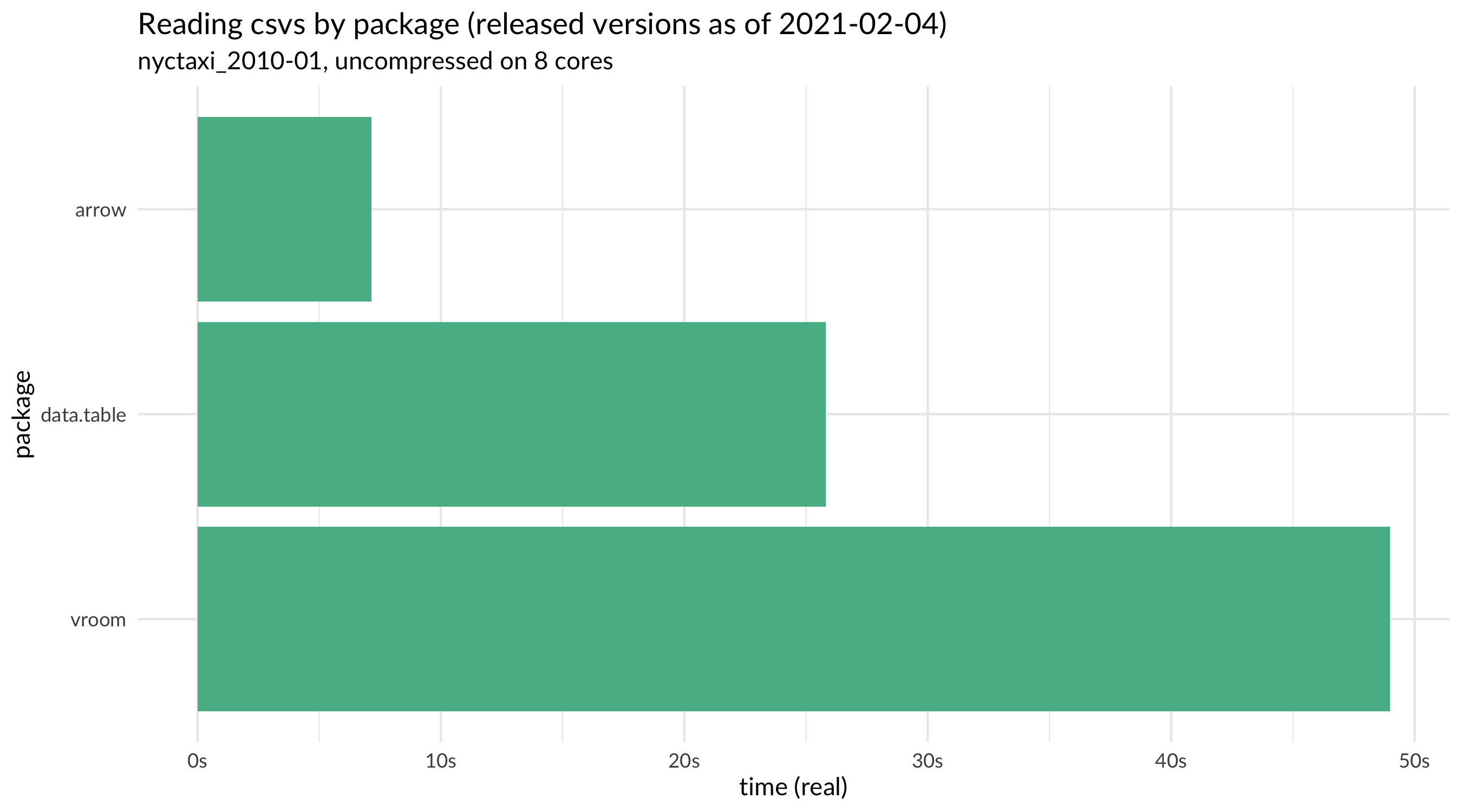
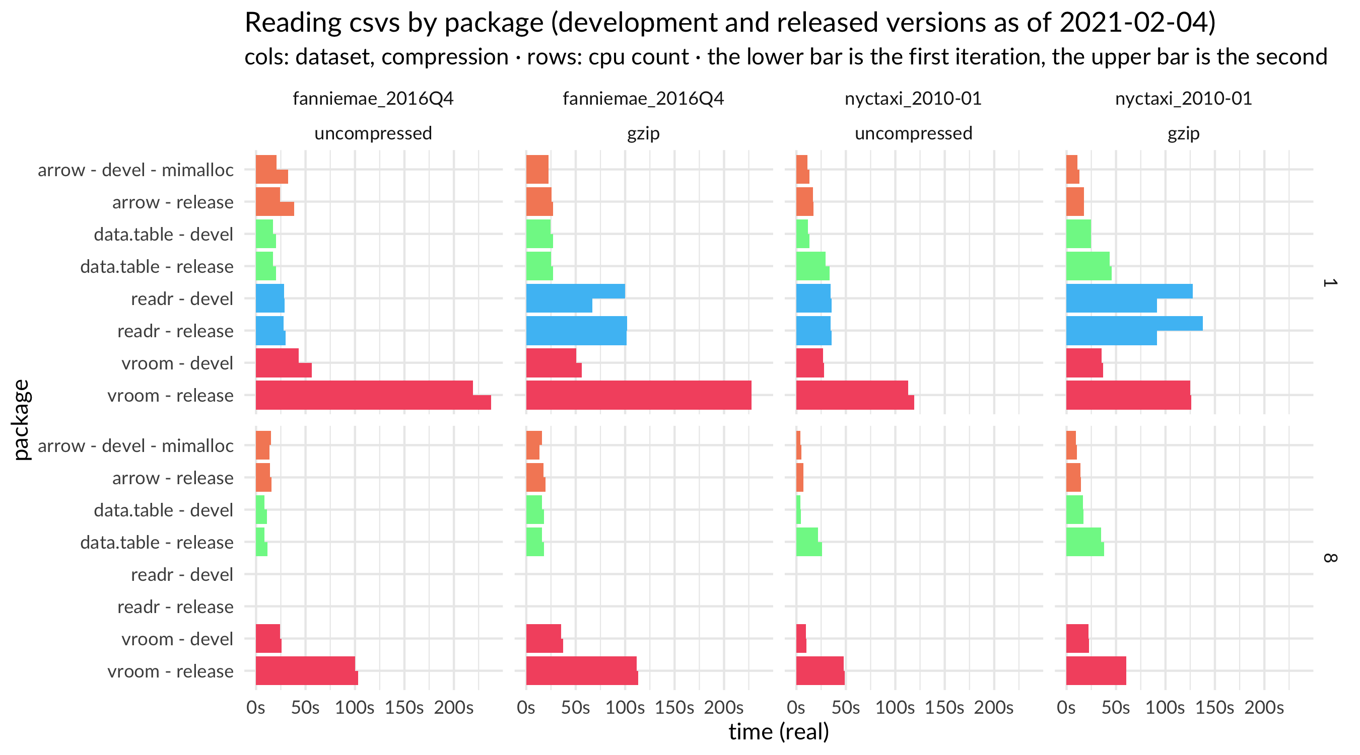
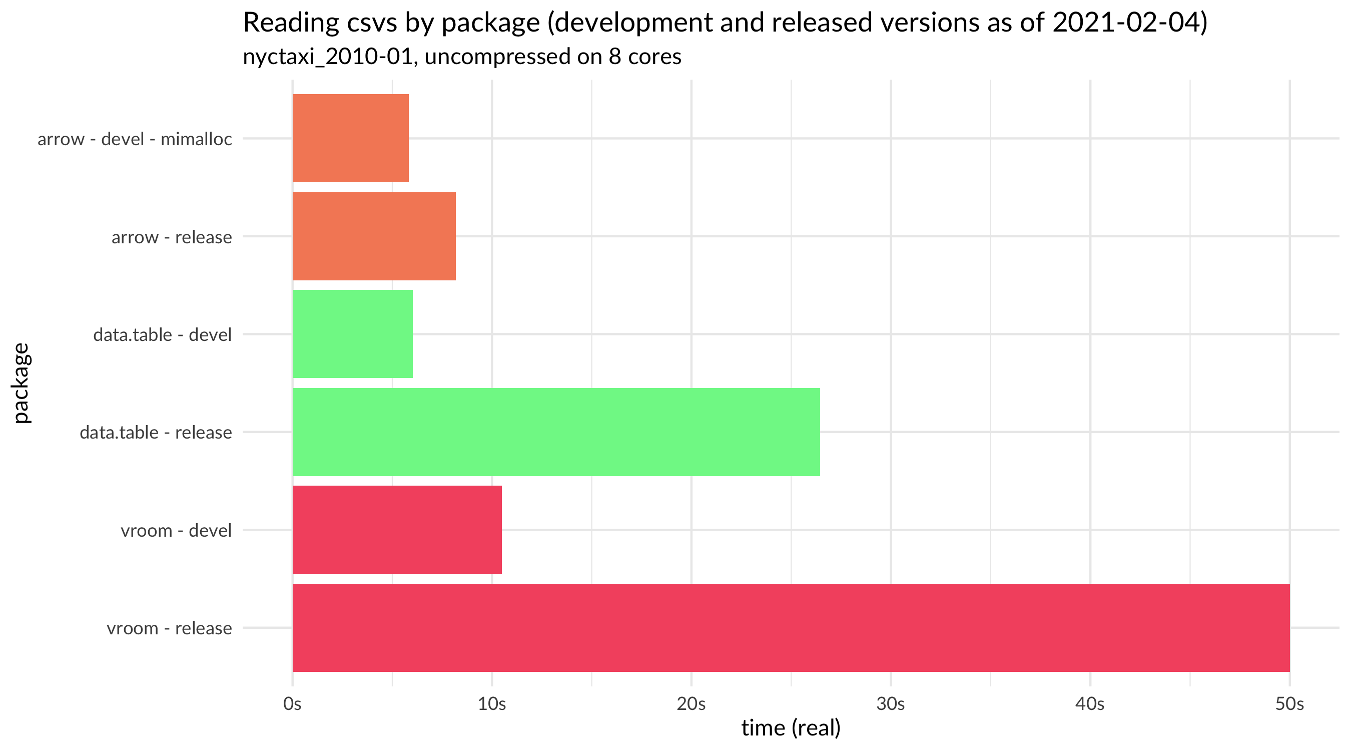
Looking at the three multi-core capable packages with their CRAN-released versions as of February 4, 2021, we see the following:

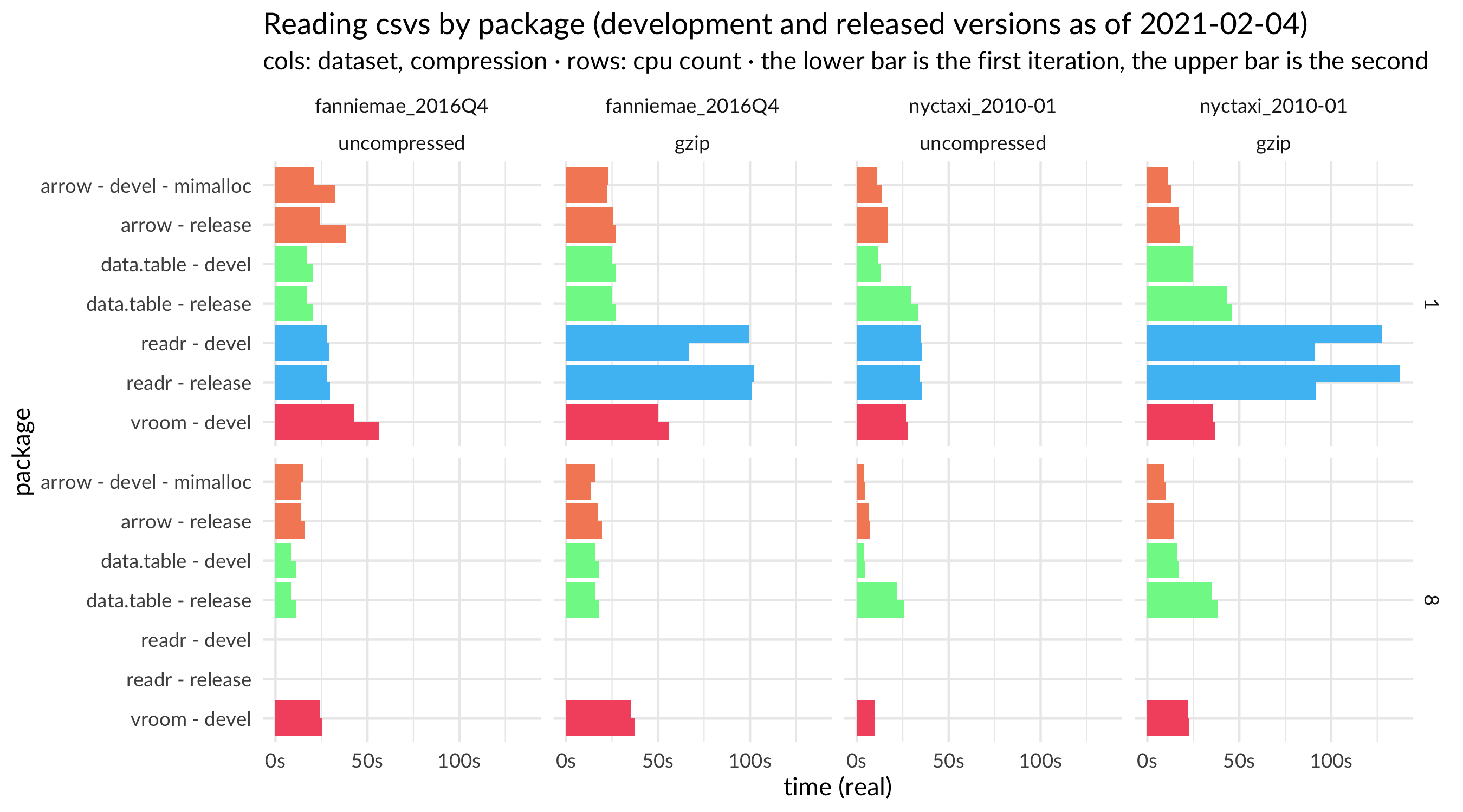
We also have a plot of full results, including with different numbers of cores, compression, and a different dataset.

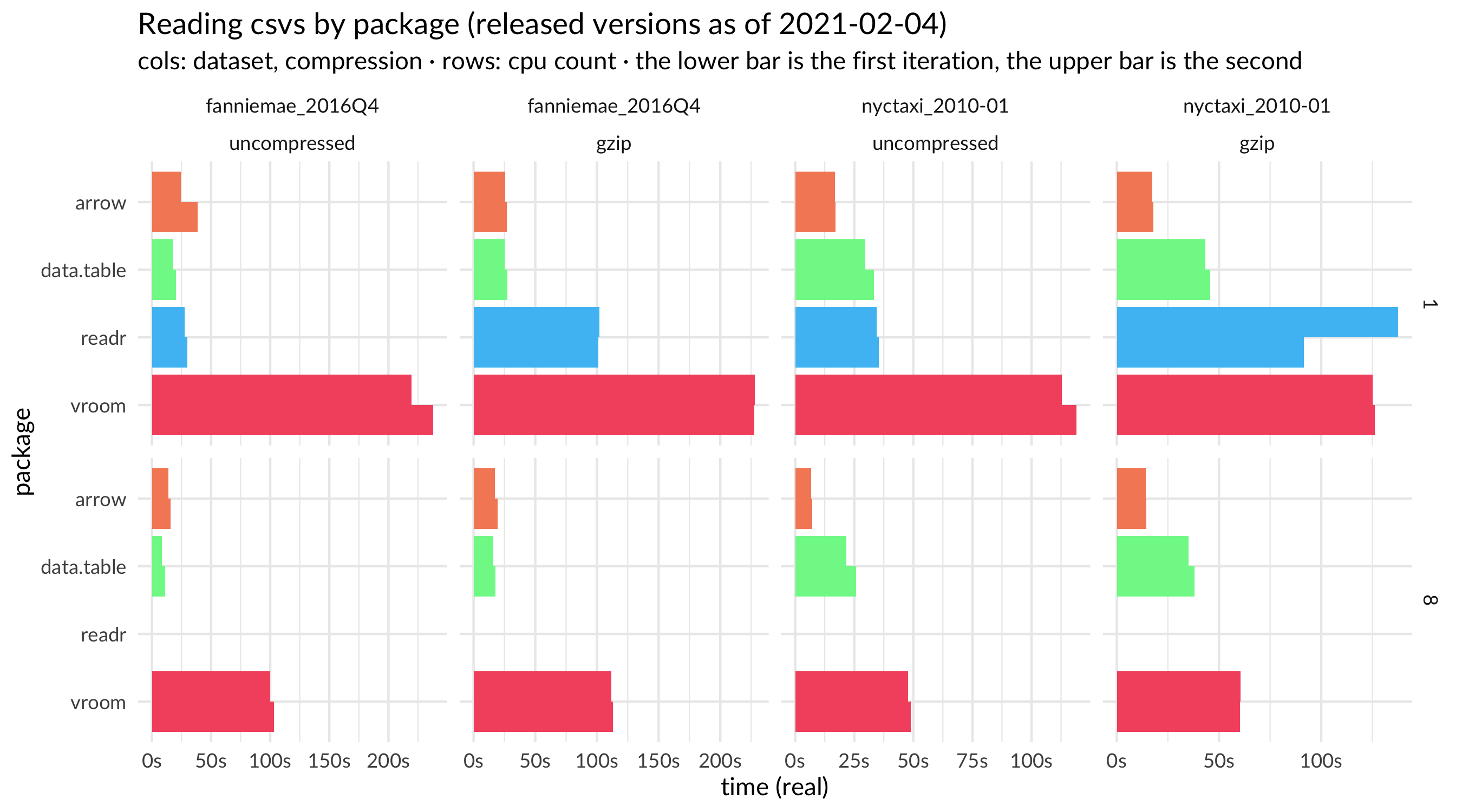
This confirms the finding from the original presentation: when reading a NYC taxi data file, {arrow} is about three times faster than {data.table} and {vroom}. Oddly, {vroom} was slightly faster than {data.table} in the August analysis but appears to take twice as long to read the file now. We’ll come back to that finding later.

Examining the full set of results from the August analysis, it seemed that Arrow’s exceptional performance could be accounted for by, among other factors, string data handling and memory allocation. We wanted to use our new benchmarking tools to explore those questions further.

String data

The {vroom} benchmarks have a few variations that test all-numeric and all-string (character) data of different shapes and sizes, and in the previous analysis, it appeared that {arrow}’s CSV reader particularly excelled at large files with lots of string data. This led us to suspect that the efficiency of Arrow format’s string data type may be an important explanation for the reader’s performance.

Under the hood, a character vector in R (a STRSXP) is a vector of CHARSXPs, each of which contains a pointer to a value in a global string pool and an encoding value. In Arrow, a string Array is essentially a big binary blob plus an array of integer offsets into it. In R-speak, c("This", "is", "a", "String", "Array") is represented something like ThisisaStringArray plus c(0, 4, 6, 7, 13, 18). This is a more compact representation with some nice properties for accessing elements within it. It’s possible that {arrow} is able to use this format as an intermediate representation and assemble R character vectors faster than R itself can. This may sound hard to believe, but we’ve observed similar results elsewhere.

Benchmark results tell us how long a task took to complete, but they don’t tell us exactly where all of that time was spent; that’s what profiling is for. However, {arrowbench} can show us what happens if we change a line of code across different versions, and from this we can see what happens if we suddenly stop taking advantage of the efficiencies of the Arrow string data type.

We unintentionally did an “experiment” that made string data conversion from Arrow to R slower in the 2.0 release. In some internal refactoring, we had unintentionally made the code that creates R character vectors less efficient by making it scan to infer the length of each element. This is not necessary when converting from Arrow because the string Array’s offsets tell us exactly how long each element is without having to recompute it. Fixing this restored the performance.

Looking at CSV read performance across released versions, we can see this anomaly pop up in the 2.0 release, and from comparing the time it takes to create an Arrow Table with the time to create an R data.frame, it is clear that the problem is located in the Arrow-to-R conversion step.

Plot of more results

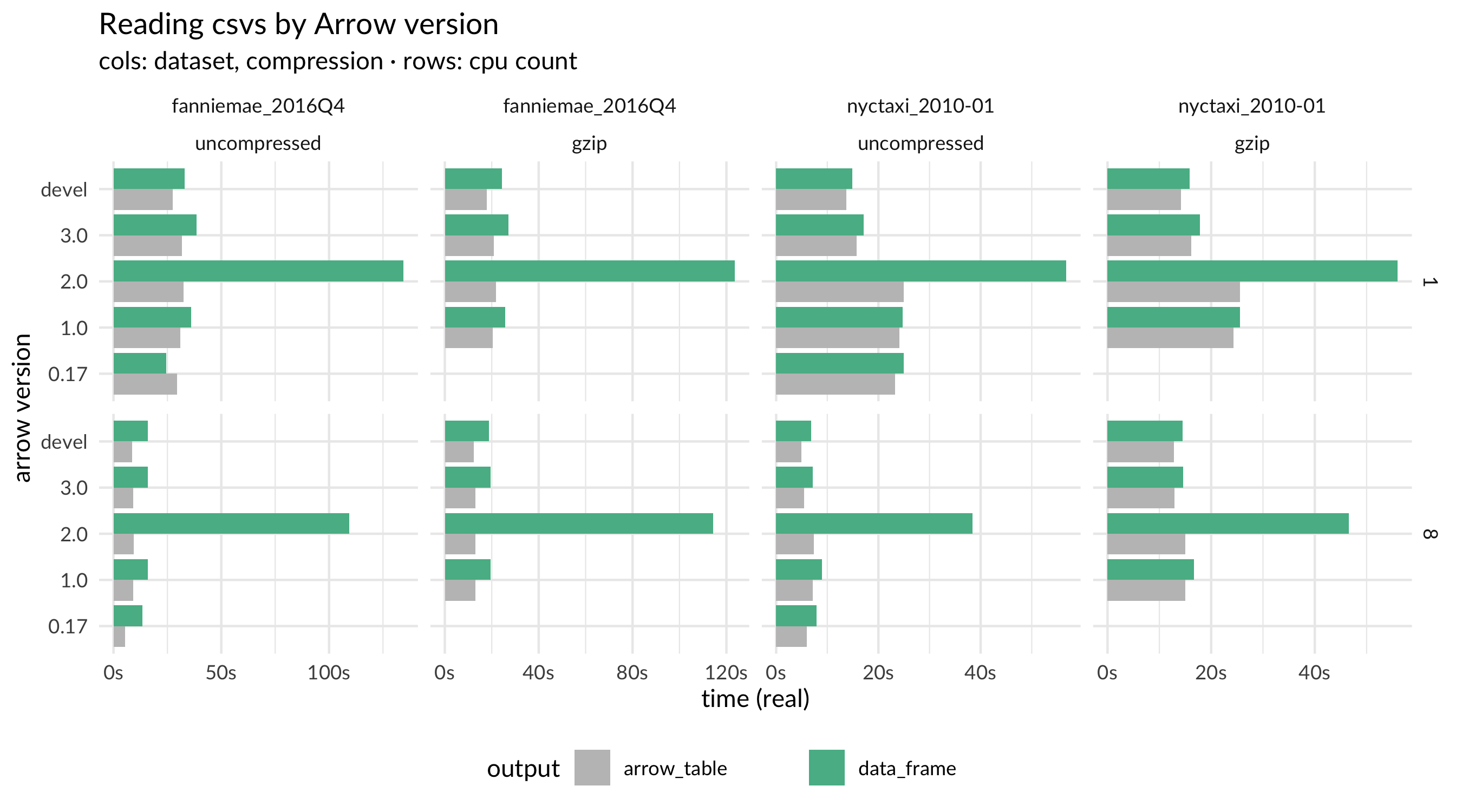
Performance regressions like these are exactly the reason we’re investing in benchmarking tools and monitoring. Our goal is to prevent slowdowns like these from getting released in the future.

Memory allocators

In order to read data in, software has to request memory from the system and allocate it, assigning objects and vectors into it. When allocating lots of memory, as we do in reading these large files in, issues such as fragmentation and multithreaded access can have significant performance implications. For this reason, a number of alternative malloc implementations exist. By default, {arrow} uses jemalloc except on Windows, where it uses mimalloc because jemalloc is not supported.

To explore how much of a performance boost we were getting from jemalloc, we took advantage of a feature in {arrow} 3.0.0 that lets you switch memory allocators by setting an environment variable. We could parametrize {arrowbench} to compare Arrow’s results using jemalloc or the system’s malloc.

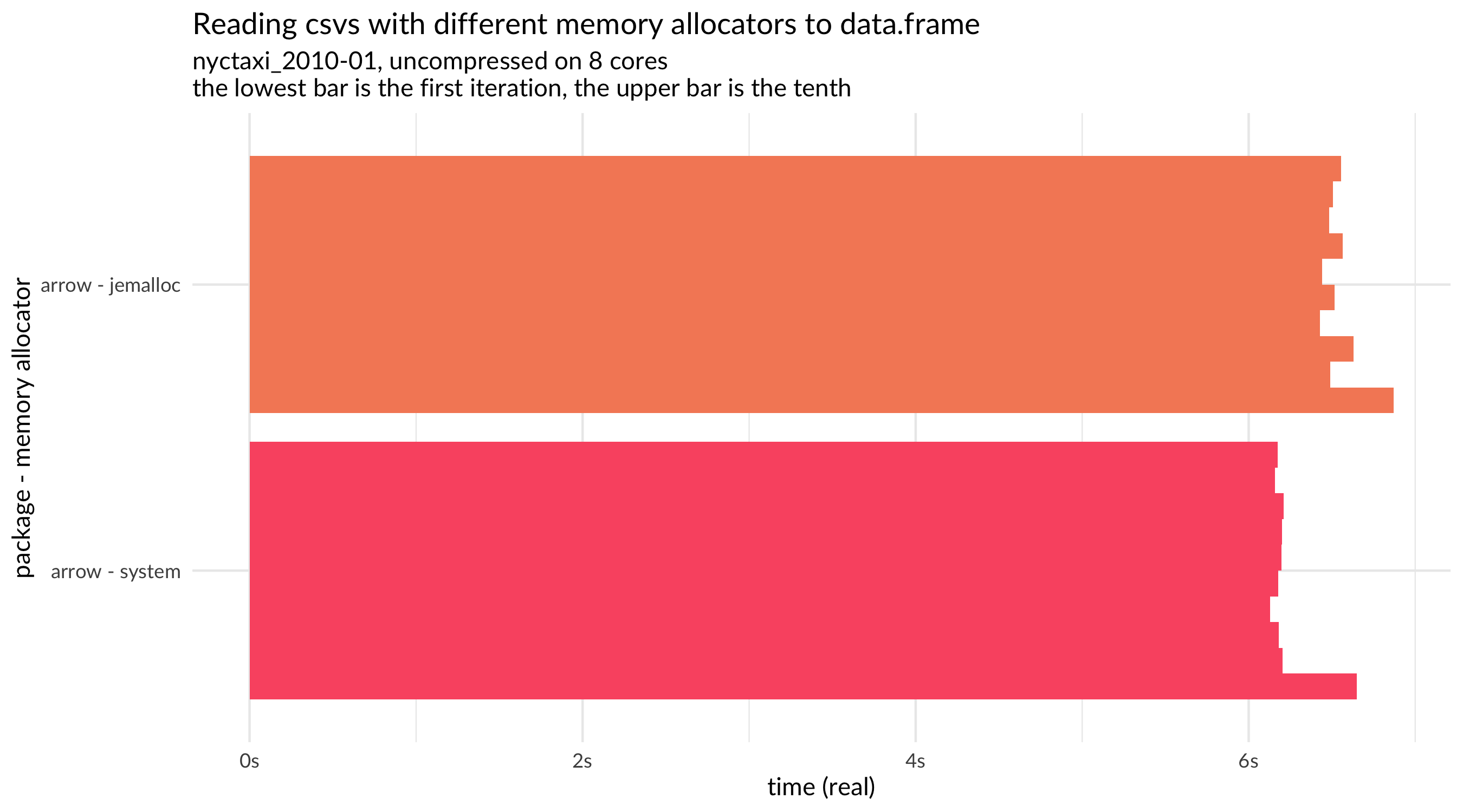
It turned out that, at least on this machine and on this workload, jemalloc wasn’t much better than the system allocator: in fact, it seemed worse. We also noticed an odd pattern in the results across multiple runs (iterations) of the same benchmark. While most benchmarks were a bit slower on the first run and then stable across subsequent runs, the results with jemalloc when reading in an Arrow Table got progressively slower (see the plot below). This was further strange because it didn’t persist when we pull data into R (which is what happens in the plot above).

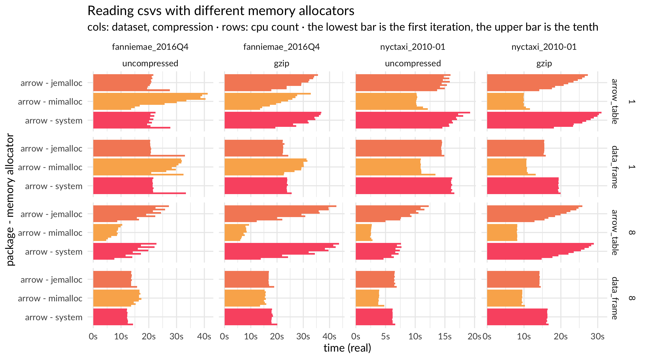
After some investigation, we isolated the cause and determined that it is specific to macOS. This led us to wonder whether mimalloc was a better alternative on macOS (or on more platforms as well). Adding mimalloc to the benchmark parameters, we see that it is indeed noticeably faster, a full second faster on reading this CSV.

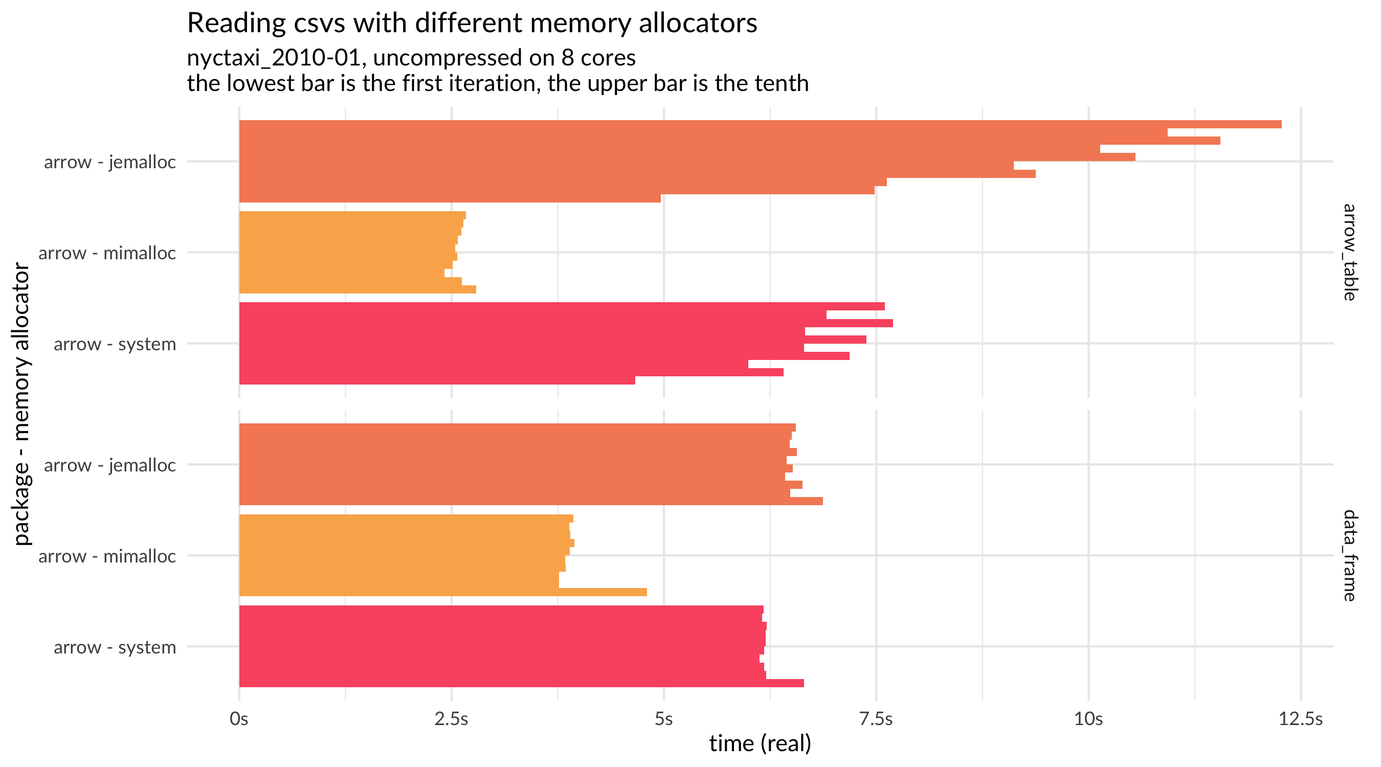
Plot of results for different memory allocators

Using benchmarks to guide development decisions

As we just learned, the choice of memory allocator has meaningful implications for performance, and at least on macOS, mimalloc seems to significantly speed up this workflow. It’s worth more analysis to see whether the same pattern holds on other workflows and on other platforms; there’s also a new release of mimalloc that may be even faster. Fortunately, we now have these benchmarking tools that help us parametrize our analyses and easily explore a range of alternatives. Using these tools, we can make technical decisions about performance based on evidence rather than conjecture.

It’s also worth noting that since we’re testing non-{arrow} packages for reference, we’re also able to detect changes in performance in those other packages and can share that information to help those maintainers improve their packages. Indeed, one result that surprised us was that the recently released 1.4 version of {vroom} seemed slower than past versions. So, we reported an issue to help {vroom}’s maintainer address it, which they quickly did.

Similarly, reacting to the August 2020 benchmark results, {data.table}’s maintainer decided to change the default timestamp parsing behavior, believing that the difference in performance with {arrow} on that particular file was due to timestamp data. Our data does show that this timestamp parsing does account for the gap between {data.table} and {arrow} on reading this file: when comparing with the Fannie Mae dataset, which does not have timestamp columns, the gap between the two readers is closed, and when we benchmark the taxi file with the development version of {data.table}, read speed is much improved.

Putting this all together, we can see the benefits of using benchmark analysis to inform development choices. This plot compares the CSV read performance of {arrow}, {data.table}, and {vroom} on both the current CRAN release versions (3.0.0, 1.13.6, and 1.4.0, respectively) along with the development versions that incorporate the changes in memory allocator ({arrow}), timestamp parsing behavior ({data.table}), and C++ value passing ({vroom}). In this particular benchmark, {arrow} and {data.table} show very similar results in their development versions; looking at the full results across multiple files and parameters, each is slightly faster in some circumstances. The results show that we can expect noticeable performance improvements in the next releases of all three packages.

Plot of full results

Plot of full results for all packages except vroom release to better show the other comparisons

Looking ahead

As should be clear from this discussion, we are firmly pro-benchmark: they can be very useful in guiding technical decisions and ensuring quality of the software we write. That said, it’s important to be clear about what benchmarks like these tell us and what they don’t. A good benchmark is like a scientific experiement: we aim to hold everything constant (hardware, inputs, settings) except for the code we’re comparing so that we can attribute any measured differences to the code that was run.

Hence, a well designed benchmark has strong internal validity—we can trust the inference that the difference in code caused the difference in performance—but that is distinct from external validity—how these results generalize outside the experimental context. Indeed, many of the things we can do to increase internal validity, such as running multiple iterations, running everything in a fresh process, or running on dedicated hardware, can add to the laboratory-like nature of the research, separating it further from the real world.

There are some things we’ve done with {arrowbench} to keep the research close to real world use. We’re focusing on real datasets, not generated data, and we are testing on multiple datasets with different characteristics—and have the ability to add more interesting datasets. Even so, every benchmark result should be read with a “your mileage may vary” disclaimer and never a guarantee that you’ll experience the exact same numbers on every dataset on every machine.

We take inspiration from that caveat, though. We’re curious how your mileage varies, and we’re excited to have better tooling to monitor performance and to investigate these kinds of questions. Indeed, one of the hardest parts of writing this post was deciding which questions to include and which questions we should mark as to-dos for our future selves to answer. Expect to see more blog posts from us that explore the performance of other key Arrow workloads and delve into the quirks we discover along the way.

---

1. Update March 2021 The repo was originally hosted by the ursa-labs organizatoin on github, it has since been moved to the ursacomputing organization. The URLs to the repository (and only these URLs) have been changed to reflect the new location. ↩︎

2. It is also an indication of speed ups that can be gained with Arrow-native workflows. We are hard at work implementing native compute in Arrow such that for many workloads the conversion from Arrow Tables to R data structures can be deferred or avoided completely. ↩︎

3. Since we’re running on a different machine, with slightly newer versions of all packages, and with a different taxi data file (January 2010 vs. January 2013), we should not directly compare the read times from this analysis with those from August 2020. ↩︎